


Measuring risk: The standard model
With 20% declines occurring, on average, every decade or so, you'd think that the standard risk models that investors use to make their asset-allocation decisions would assign a significant probability t
hat these events will occur. Think again. To see why, we need to look at the history of how these models were formed.
To help make sense of the highly complex capital markets, financial economists in 1960s and 1970s developed a set of mathematical models of the markets that are used to this day throughout the investment profession. The best known of these models are the capital asset pricing model of expected returns and the Black-Scholes option pricing model. These models' creators have won the Nobel Prize in economics for their path-breaking work. Each of these models starts by making an assumption about the statistical distribution of stock market returns. The CAPM assumes that returns follow a normal, or bell-shaped, distribution. The Black- Scholes model assumes that returns follow a lognormal distribution.4
With these standard models, the primary measure of risk is standard deviation. If returns follow a normal distribution, the chance that a return would be more than three standard deviations below average would be a trivial 0.135%. Since January 1926, we have 996 months of stock market data; 0.135% of 996 is 1.34--that is, there should be only one or two occurrences of such event.
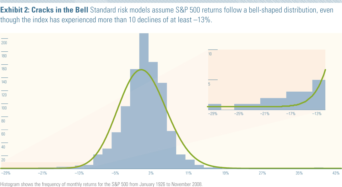
But the record of the stock market tells a different story. The monthly returns of the S&P 500 have been more than three standard deviations below average 10 times since 1926. In other words, the standard models assign meaninglessly small probabilities to extreme events that occur five to 10 times more than the models predict.
We can illustrate the problem further by overlaying a lognormal model of returns over a histogram of monthly total returns on the S&P 500 (Exhibit 2). The model says that declines of more than negative 13% have almost no chance of happening--yet they have occurred at least 10 times since 1926.
Footnotes:
4. For returns to follow a lognormal distribution means that logarithm one plus the return in decimal follows a normal distribution.
This article first appeared in the February/March 2009 issue of Morningstar Advisor Magazine.


